Growing Cell Structures

 

• Common Properties and Notational Conventions
• Java implementation not (yet) available

This model (Fritzke, 1994a) is rather similar to the growing neural gas model

. The main difference is that the network topology is constrained to consist of k-dimensional simplices whereby k is some positive integer chosen in advance. The basic building block and also the initial configuration of each network is a k-dimensional simplex. This is, e.g., a line for k=1, a triangle for k=2, and a tetrahedron for k=3.

For a given network configuration a number of adaptation steps are used to update the reference vectors of the nodes and to gather local error information at each node.

This error information is used to decide where to insert new nodes. A new node is always inserted by splitting the longest edge emanating from the node q with maximum accumulated error. In doing this, additional edges are inserted such that the resulting structure consists exclusively of k-dimensional simplices again.

The growing cell structures learning procedure is described in the following:

1.

Choose a network dimensionality k.

Initialize the set to contain k+1 units

with reference vectors chosen randomly according to .

Initialize the connection set , such that each unit is connected to each other unit, i.e., such that the network has the topology of a k-dimensional simplex.

2.

Generate at random an input signal according to .

3.

Determine the winner s:

4.

Add the squared distancebetween the input signal and the winner unit s to a local error variable :

5.

Adapt the reference vectors of s and its direct topological neighbors towards by fractions  and , respectively, of the total distance:

Thereby, we denote with the set of direct topological neighbors of s.

6.

If the number of input signals generated so far is an integer multiple of a parameter , insert a new unit as follows:

Determine the unit q with the maximum accumulated error:

Insert a new unit r by splitting the longest edge emanating from q, say an edge leading to a unit f. Insert the connections (q,r) and (r,f) and remove the original connection (q,f). To re-build the structure such that it again consists only of k-dimensional simplices, the new unit r is also connected with all common neighbors of q and f, i.e., with all units in the set .

Interpolate the reference vector of r from the reference vectors of q and f:

Decrease the error variables of all neighbors of r by a fraction which depends on the number of neighbors of r:
 

Set the error variable of the new unit r to the mean value of its neighbors:

7.

Decrease the error variables of all units:
 

8.

If a stopping criterion (e.g., net size or some performance measure) is not yet fulfilled continue with step 2.

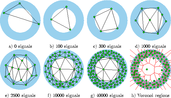
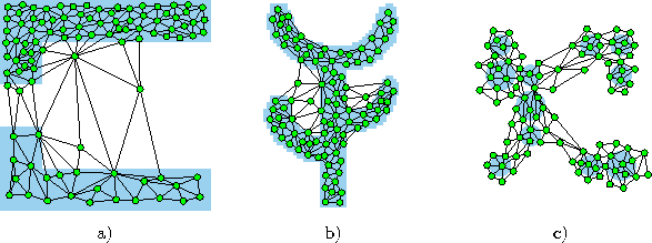
Figure 6.3 shows some stages of a simulation for a simple ring-shaped data distribution. Figure 6.4 displays the final results after 40000 adaptation steps for three other distribution. The parameters used in both simulations were: .

 
Figure 6.3:   Growing cell structures simulation sequence for a ring-shaped uniform probability distribution. a) Initial state. b-f) Intermediate states. g) Final state. h) Voronoi tessellation corresponding to the final state. Per construction the network structure always consists of hypertetrahedrons (triangles in this case).

 
Figure:   Growing cell structures simulation results after 40000 input signals for three different probability distributions (described in the caption of figure 4.4).