The models described in this report share several architectural properties which are described in this chapter. For simplicity, we will refer to any of these models as network even if the model does not belong to what is usually understood as ``neural network''.
Each network consists of a set of N units:
![]()
Each unit c has an associated reference vector
![]()
indicating its position or receptive field center in input space.
Between the units of the network there exists a (possibly empty) set
![]()
of neighborhood connections which are unweighted
and symmetric:
![]()
These connections have nothing to do with the weighted connections
found, e.g., in multi-layer perceptrons (Rumelhart et al., 1986). They are
used in some methods to extend the adaptation of the winner (see
below) to some of its topological neighbors.
For a unit c we denote with ![]() the set of its direct topological
neighbors:
the set of its direct topological
neighbors:
![]()
The n-dimensional input signals are assumed to be generated either according to a continuous probability density function
![]()
or from a finite training data set
![]()
For a given input signal ![]() the winner
the winner ![]() among the
units in
among the
units in ![]() is defined as the unit with the nearest reference
vector
is defined as the unit with the nearest reference
vector
![]()
whereby ![]() denotes the Euclidean vector norm.
In case of a tie among several units one of them is chosen to be the
winner by throwing a fair dice. In some cases we will denote the
current winner simply by s (omitting the dependency on
denotes the Euclidean vector norm.
In case of a tie among several units one of them is chosen to be the
winner by throwing a fair dice. In some cases we will denote the
current winner simply by s (omitting the dependency on ![]() ). If
not only the winner but also the second-nearest unit or even more
distant units are of interest, we denote with
). If
not only the winner but also the second-nearest unit or even more
distant units are of interest, we denote with ![]() the i-nearest
unit (
the i-nearest
unit (![]() is the winner,
is the winner, ![]() is the second-nearest unit, etc.).
is the second-nearest unit, etc.).
Two fundamental and closely related concepts from computational geometry are important to understand in this context. These are the Voronoi Tessellation and the Delaunay Triangulation:
Given a set of vectors ![]() in
in ![]() (see figure
2.1 a), the Voronoi Region
(see figure
2.1 a), the Voronoi Region ![]() of a particular
vector
of a particular
vector ![]() is defined as the set of all points in
is defined as the set of all points in ![]() for which
for which
![]() is the nearest vector:
is the nearest vector:
![]()
In order for each data point to be associated to exactly one Voronoi region we define (as previously done for the winner) that in case of a tie the corresponding point is mapped at random to one of the nearest reference vectors. Alternatively, one could postulate general positions for all data points and reference vectors in which case a tie would have zero probability.
It is known, that each Voronoi region ![]() is a convex area, i.e.
is a convex area, i.e.
![]()
The partition of ![]() formed by all Voronoi polygons is called
Voronoi Tessellation or Dirichlet
Tessellation (see figure
2.1 b). Efficient algorithms
to compute it are only known for two-dimensional data sets
(Preparata and Shamos, 1990). The concept itself, however, is applicable to
spaces of arbitrarily high dimensions.
formed by all Voronoi polygons is called
Voronoi Tessellation or Dirichlet
Tessellation (see figure
2.1 b). Efficient algorithms
to compute it are only known for two-dimensional data sets
(Preparata and Shamos, 1990). The concept itself, however, is applicable to
spaces of arbitrarily high dimensions.
If one connects all pairs of points for which the respective Voronoi regions share an edge (an (n-1)-dimensional hyperface for spaces of dimension n) one gets the Delaunay Triangulation (see figure 2.1 c). This triangulation is special among all possible triangulation in various respects. It is, e.g., the only triangulation in which the circumcircle of each triangle contains no other point from the original point set than the vertices of this triangle. Moreover, the Delaunay triangulation has been shown to be optimal for function interpolation (Omohundro, 1990). The competitive Hebbian learning method generates a subgraph of the Delaunay triangulation which is limited to those areas of the input space where data is found.
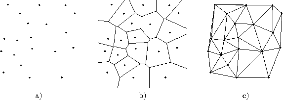
Figure 2.1: a) Point set in ![]() , b) corresponding Voronoi tessellation, c)
corresponding Delaunay triangulation.
, b) corresponding Voronoi tessellation, c)
corresponding Delaunay triangulation.
For convenience we define the Voronoi Region of a unit ![]() , as the Voronoi region of its reference vector:
, as the Voronoi region of its reference vector:
![]()
In the case of a finite input data set ![]() we denote for a unit c with the term Voronoi Set the subset
we denote for a unit c with the term Voronoi Set the subset ![]() of
of ![]() for which c is the winner (see figure 2.2):
for which c is the winner (see figure 2.2):
![]()
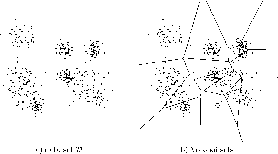
Figure 2.2:
An input data set ![]() is shown (a) and the partition of
is shown (a) and the partition of ![]() into Voronoi sets for a particular set of reference vectors (b). Each Voronoi set contains the data points within the corresponding Voronoi field.
into Voronoi sets for a particular set of reference vectors (b). Each Voronoi set contains the data points within the corresponding Voronoi field.