Growing grid is another incremental network. The basic principles used also in growing cell structures and growing neural gas are applied with some modifications to a rectangular grid. Alternatively, growing grid can be seen as an incremental variant of the self-organizing feature map.
The model has two distinct phases, a growth phase and a fine-tuning phase. During the growth phase a rectangular network is built up starting from a minimal size by inserting complete rows and columns until the desired size is reached or until a performance criterion is met. Only constant parameters are used in this phase. In the fine-tuning phase the size of the network is not changed anymore and a decaying learning rate is used to find good final values for the reference vectors.
As for the self-organizing map, the network structure is a
two-dimensional grid (![]() ). This grid is initially set to
). This grid is initially set to
![]() structure. Again, the distance on the grid is used to
determine how strongly a unit
structure. Again, the distance on the grid is used to
determine how strongly a unit ![]() is adapted when the unit
is adapted when the unit ![]() is the winner. The distance measure used is the
is the winner. The distance measure used is the ![]() -norm
-norm
![]()
Also the function used to determine the adaptation strength for a unit
r given that s is the winner is the same as for the self-organizing feature map:
![]()
The width parameter ![]() , however, remains constant throughout the
whole simulation. It is chosen relatively small compared to the values
usually used at the beginning for the self-organizing feature map. One can note that as the
growing grid network grows, the fraction of all units which is adapted
together with the winner decreases. This is also the case in the
self-organizing feature map but is achieved there with a constant network size and a
decreasing neighborhood width.
The complete growing grid algorithm is the following:
, however, remains constant throughout the
whole simulation. It is chosen relatively small compared to the values
usually used at the beginning for the self-organizing feature map. One can note that as the
growing grid network grows, the fraction of all units which is adapted
together with the winner decreases. This is also the case in the
self-organizing feature map but is achieved there with a constant network size and a
decreasing neighborhood width.
The complete growing grid algorithm is the following:
Growth Phase
Initialize the connection set ![]() to form a rectangular
to form a rectangular ![]() grid.
grid.
Initialize the time parameter t:
![]()
Fine-tuning Phase
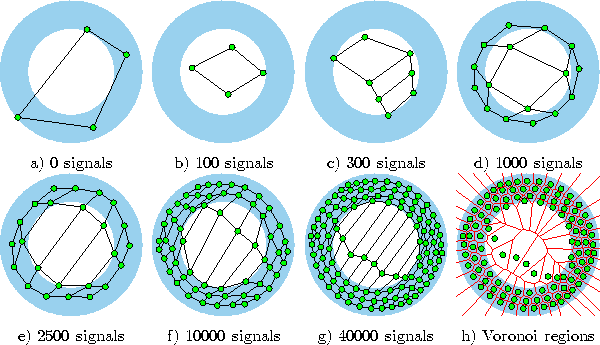
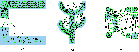
Figure 6.5 shows some stages of a simulation for a simple ring-shaped data distribution. Figure 6.6 displays the final results after 40000 adaptation steps for three other distribution.
The parameters used for the growth phase were: ![]() . The parameters for the fine-tuning phase were:
. The parameters for the fine-tuning phase were: ![]() and
and ![]() unchanged,
unchanged, ![]() .
.

Figure 6.5: Growing grid simulation sequence for a ring-shaped uniform probability distribution. a) Initial state. b-f) Intermediate states. g) Final state. h) Voronoi tessellation corresponding to the final state.

Figure: Growing grid simulation results after 40000 input signals for three different probability distributions (described in the caption of figure 4.4). One can note that in a) the chosen topology (![]() ) has a rather extreme height/width ratio which matches well the distribution at hand. Depending on initial conditions however, also other topologies occur in simulations for this distribution. b),c) Also these topologies deviate from the square shape usually given to self-organizing maps. For the cactus a (
) has a rather extreme height/width ratio which matches well the distribution at hand. Depending on initial conditions however, also other topologies occur in simulations for this distribution. b),c) Also these topologies deviate from the square shape usually given to self-organizing maps. For the cactus a (![]() ) and for the mixture distribution a (
) and for the mixture distribution a (![]() ) topology was automatically selected by the algorithm.
) topology was automatically selected by the algorithm.
If one compares the growing grid algorithm with the other incremental
methods growing cell structures and growing neural gas then a difference (apart from the topology)
is that no counter variables are redistributed when new units are
inserted. Instead, all ![]() -values are set to zero after a row or
column has been inserted. This means, that all statistical information
about winning frequencies is discarded after an insertion. Therefore,
to gather enough statistical evidence where to insert new units the
next time, the number of adaptation steps per insertion step
must be proportional to the network size (see equation 6.31).
This simplifies the algorithm but increases the computational
complexity. The same could in principle be done with growing neural gas and growing cell structures
effectively eliminating the need to re-distribute accumulated
information after insertions at the price of increased computational
complexity.
-values are set to zero after a row or
column has been inserted. This means, that all statistical information
about winning frequencies is discarded after an insertion. Therefore,
to gather enough statistical evidence where to insert new units the
next time, the number of adaptation steps per insertion step
must be proportional to the network size (see equation 6.31).
This simplifies the algorithm but increases the computational
complexity. The same could in principle be done with growing neural gas and growing cell structures
effectively eliminating the need to re-distribute accumulated
information after insertions at the price of increased computational
complexity.
The parameter ![]() which governs the neighborhood range has the
function of a regularizer. If it is set to large values, then
neighboring units are forced to have rather similar reference vectors
and the layout of the network (when projected to input space) will
appear very regular but not so well adapted to the underlying data
distribution
which governs the neighborhood range has the
function of a regularizer. If it is set to large values, then
neighboring units are forced to have rather similar reference vectors
and the layout of the network (when projected to input space) will
appear very regular but not so well adapted to the underlying data
distribution ![]() . Smaller values for
. Smaller values for ![]() give the units
more possibilities to adapt independently from each other. As
give the units
more possibilities to adapt independently from each other. As ![]() is set more and more to zero the growing grid algorithm (apart from the
insertions) approaches hard competitive learning.
is set more and more to zero the growing grid algorithm (apart from the
insertions) approaches hard competitive learning.
Similar to the self-organizing feature map the growing grid algorithm can easily be applied to network structures of other dimensions than two. Actually useful, however, seem only the cases of one- and three-dimensional networks since networks of higher dimensionality can not be visualized easily.