If the learning rate is constant, i.e.
From (4.8) and (4.11) it is obvious that
the influence of past input signals decays exponentially fast with the
number of further input signals for which c is winner (see also figure
4.2). The most recent input signal, however, always
determines a fraction ![]() of the current value of
of the current value of ![]() . This
has two consequences. First, such a system stays adaptive and is
therefore in principle able to follow also non-stationary signal
distribution
. This
has two consequences. First, such a system stays adaptive and is
therefore in principle able to follow also non-stationary signal
distribution ![]() . Second (and for the same reason), there is no
convergence. Even after a large number of input signals the current
input signal can cause a considerable change of the reference vector
of the winner. A typical behavior of such a system in case of a
stationary signal distribution is the following: the reference vectors drift
from their initial positions to quasi-stationary positions where
they start to wander around a dynamic equilibrium. Better
quasi-stationary positions in terms of mean square error are
achieved with smaller learning rates. In this case, however, the
system also needs more adaptation steps to reach the
quasi-stationary positions.
. Second (and for the same reason), there is no
convergence. Even after a large number of input signals the current
input signal can cause a considerable change of the reference vector
of the winner. A typical behavior of such a system in case of a
stationary signal distribution is the following: the reference vectors drift
from their initial positions to quasi-stationary positions where
they start to wander around a dynamic equilibrium. Better
quasi-stationary positions in terms of mean square error are
achieved with smaller learning rates. In this case, however, the
system also needs more adaptation steps to reach the
quasi-stationary positions.

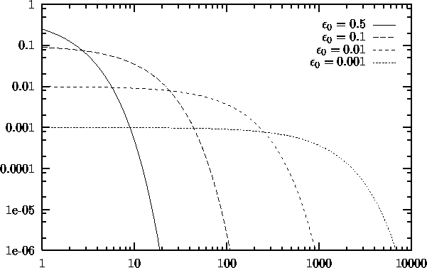
Figure 4.2: Influence of an input signal ![]() on the vector of its winner s as a function of the number of following input signals for which s is winner (including
on the vector of its winner s as a function of the number of following input signals for which s is winner (including ![]() ). Results for different constant adaptation rates are shown. The respective
section with the x-axis indicates how many signals are needed until the influence of
). Results for different constant adaptation rates are shown. The respective
section with the x-axis indicates how many signals are needed until the influence of ![]() is below
is below ![]() . For example if the learning rate
. For example if the learning rate ![]() is set to 0.5, about 10 additional signals (the section with the x-axis is near 11) are needed to let this happen.
is set to 0.5, about 10 additional signals (the section with the x-axis is near 11) are needed to let this happen.
If the distribution is non-stationary then the information about the
non-stationarity (how rapidly does the distribution change) can be
used to set an appropriate learning rate. For rapidly changing
distributions relatively large learning rates should be used and vice
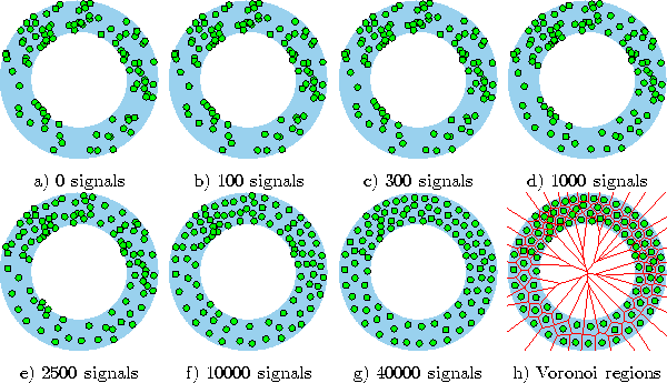
versa. Figure 4.3 shows some stages of a simulation for a simple ring-shaped data distribution. Figure 4.4 displays the final results after 40000 adaptation steps for three other distribution. In both cases a constant learning rate
![]() was used.
was used.

Figure 4.3: Hard competitive learning simulation sequence for a ring-shaped uniform probability distribution. A constant adaptation rate was used. a) Initial state. b-f) Intermediate states. g) Final state. h) Voronoi tessellation corresponding to the final state.

Figure 4.4: Hard competitive learning simulation results after 40000 input signals for three different probability distributions. A constant learning rate was used. a) This distribution is uniform within both shaded areas. The probability density, however, in the upper shaded area is 10 times as high as in the lower one. b) The distribution is uniform in the shaded area. c) In this distribution each of the 11 circles indicates the standard deviation of a Gaussian kernel which was used to generate the data. All Gaussian kernels have the same a priori probability.