Growing Neural Gas

• Common Properties and Notational Conventions
• Java implementation
  

This method (Fritzke, 1994b, 1995a) is different from the previously described models since the number of units is changed (mostly increased) during the self-organization process. The growth mechanism from the earlier proposed growing cell structures (Fritzke, 1994a) and the topology generation of competitive Hebbian learning (Martinetz and Schulten, 1991) are combined to a new model. Starting with very few units new units are inserted successively. To determine where to insert new units, local error measures are gathered during the adaptation process. Each new unit is inserted near the unit which has accumulated most error. The complete growing neural gas algorithm is the following:

1.

Initialize the set to contain two units and

with reference vectors chosen randomly according to .

Initialize the connection set , , to the empty set:

2.

Generate at random an input signal according to .

3.

Determine the winner and the second-nearest unit by

and

4.

If a connection between and does not exist already, create it:

Set the age of the connection between and to zero (``refresh'' the edge):

5.

Add the squared distance between the input signal and the winner to a local error variable:

6.

Adapt the reference vectors of the winner and its direct topological neighbors by fractions  and , respectively, of the total distance to the input signal:

Thereby (see equation 2.5) is the set of direct topological neighbors of .

7.

Increment the age of all edges emanating from :

8.

Remove edges with an age larger than . If this results in units having no more emanating edges, remove those units as well.

9.

If the number of input signals generated so far is an integer multiple of a parameter , insert a new unit as follows:

Determine the unit q with the maximum accumulated error:

Determine among the neighbors of q the unit f with the maximum accumulated error:

Add a new unit r to the network and interpolate its reference vector from q and f.

Insert edges connecting the new unit r with units q and f, and remove the original edge between q and f:

Decrease the error variables of q and f by a fraction :

Interpolate the error variable of r from q and f:

10.

Decrease the error variables of all units:

11.

If a stopping criterion (e.g., net size or some performance measure) is not yet fulfilled continue with step 2.

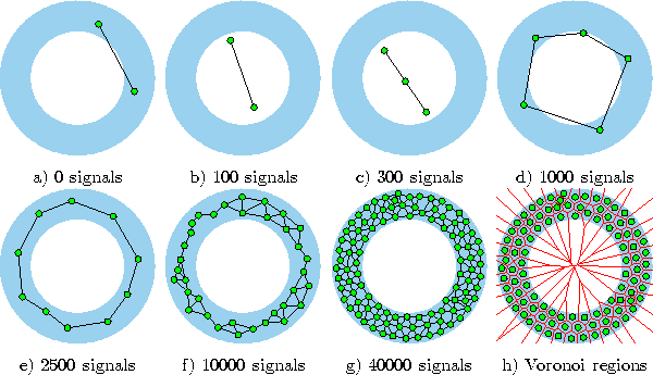
Figure 5.7 shows some stages of a simulation for a simple ring-shaped data distribution. Figure 5.8 displays the final results after 40000 adaptation steps for three other distribution. The parameters used in both simulations were: , , , , , .

 
Figure 5.7:   Growing neural gas simulation sequence for a ring-shaped uniform probability distribution. a) Initial state. b-f) Intermediate states. g) Final state. h) Voronoi tessellation corresponding to the final state. The maximal network size was set to 100.

 
Figure:   Growing neural gas simulation results after 40000 input signals for three different probability distributions (described in the caption of figure 4.4).