Another possibility for a decaying adaptation rate has been proposed by Ritter et al. (1991) in the context of self-organizing maps. They propose an exponential decay according to
In figure 4.7 this kind of learning rate is compared to
the harmonic series for a specific choice of parameters. In particular
at the beginning of the simulation the exponentially decaying learning
rate is considerably larger than that dictated by the harmonic series.
This can be interpreted as introducing noise to the system which is
then gradually removed and, therefore, suggests a relationship to
simulated annealing techniques (Kirkpatrick et al., 1983). Simulated
annealing gives a system the ability to escape from poor local minima
to which it might have been initialized. Preliminary experiments
comparing k-means and hard competitive learning with a learning rate
according to (4.18) indicate that the latter method is less
susceptible to poor initialization and for many data distributions
gives lower mean square error. Also small constant learning rates
usually give better results than k-means. Only in the special case that only one
reference vector exists (![]() ) it is completely impossible to
beat k-means on average, since in this case it realizes the optimal
estimator (the mean of all samples occurred so far). These
observations are in complete agreement with Darken and Moody (1990) who
investigated k-means and a number of different learning rate schedules
like constant learning rates and a learning rate which is the square
root of the rate used by k-means (
) it is completely impossible to
beat k-means on average, since in this case it realizes the optimal
estimator (the mean of all samples occurred so far). These
observations are in complete agreement with Darken and Moody (1990) who
investigated k-means and a number of different learning rate schedules
like constant learning rates and a learning rate which is the square
root of the rate used by k-means (![]() ). Their
results indicate that if k is larger than 1, then k-means is inferior to
the other learning rate schedules. In the examples they give the
difference in distortion error is up to two orders of magnitude.
). Their
results indicate that if k is larger than 1, then k-means is inferior to
the other learning rate schedules. In the examples they give the
difference in distortion error is up to two orders of magnitude.
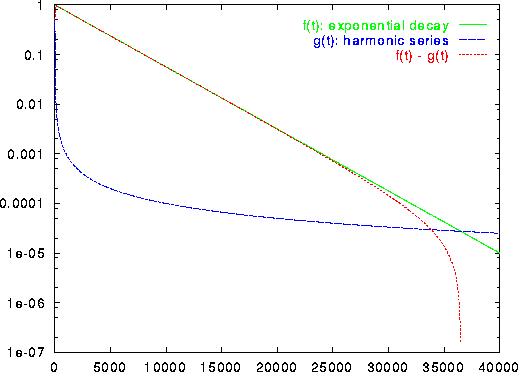
Figure 4.7: Comparison of the exponentially decaying learning function ![]() and the harmonic series g(t) = 1/t for a particular set of parameters (
and the harmonic series g(t) = 1/t for a particular set of parameters (![]() ). The displayed difference between the two learning rates can be interpreted as noise which in the case of an exponentially decaying learning rate is introduced to the system and then gradually removed.
). The displayed difference between the two learning rates can be interpreted as noise which in the case of an exponentially decaying learning rate is introduced to the system and then gradually removed.
Figure 4.8 shows some stages of a simulation for a simple ring-shaped data distribution. Figure 4.9 displays the final results after 40000 adaptation steps for three other distribution.
The parameters used in both examples were: ![]() and
and ![]() .
.
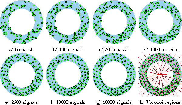
Figure 4.8: Hard competitive learning simulation sequence for a ring-shaped uniform probability distribution. An exponentially decaying learning rate was used. a) Initial state. b-f) Intermediate states. g) Final state. h) Voronoi tessellation corresponding to the final state.
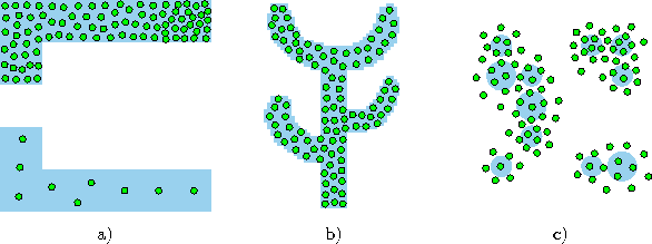
Figure: Hard competitive learning simulation results after 40000 input signals for three different probability distributions (described in the caption of figure 4.4). An exponentially decaying learning rate was used.