
One should note that the set of signals
![]() for which a particular unit c
has been winner may contain elements which lie outside the current
Voronoi region of c. The reason is that each adaptation of
for which a particular unit c
has been winner may contain elements which lie outside the current
Voronoi region of c. The reason is that each adaptation of ![]() changes the borders of the Voronoi region
changes the borders of the Voronoi region ![]() . Therefore, although
. Therefore, although
![]() represents the arithmetic mean of the signals it has been
winner for, at time t some of these signal may well lie in Voronoi
regions belonging to other units.
represents the arithmetic mean of the signals it has been
winner for, at time t some of these signal may well lie in Voronoi
regions belonging to other units.
Another important point about k-means is, that there is no strict
convergence (as is present e.g. in LBG), the reason being that the
sum of the harmonic series diverges:
![]()
Because of this divergence, even after a large number of input signals
and correspondingly low values of the learning rate ![]() arbitrarily large modifications of each input vector may occur in
principal. Such large modification, however, are very improbable and
in simulations where the signal distribution is stationary the
reference vectors usually rather quickly take on values which are not
much changed in the following. In fact, it has been shown that
k-means does converge asymptotically to a configuration where each
reference vector
arbitrarily large modifications of each input vector may occur in
principal. Such large modification, however, are very improbable and
in simulations where the signal distribution is stationary the
reference vectors usually rather quickly take on values which are not
much changed in the following. In fact, it has been shown that
k-means does converge asymptotically to a configuration where each
reference vector ![]() is positioned such that it coincides with the
expectation value
is positioned such that it coincides with the
expectation value
![]()
of its Voronoi region ![]() (MacQueen, 1965). One can note that (4.17) is
the continuous variant of the centroid condition (4.2).
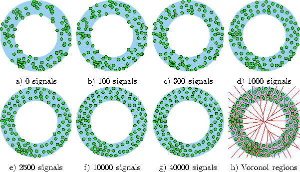
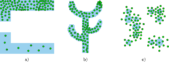
Figure 4.5 shows some stages of a simulation for a simple ring-shaped data distribution. Figure 4.6 displays the final results after 40000 adaptation steps for three other distribution.
(MacQueen, 1965). One can note that (4.17) is
the continuous variant of the centroid condition (4.2).
Figure 4.5 shows some stages of a simulation for a simple ring-shaped data distribution. Figure 4.6 displays the final results after 40000 adaptation steps for three other distribution.

Figure 4.5: k-means simulation sequence for a ring-shaped uniform probability distribution. a) Initial state. b-f) Intermediate states. g) Final state. h) Voronoi tessellation corresponding to the final state. The final distribtion of the reference vectors still reflects the clusters present in the initial state (see in particular the region of higher vector density at the lower left).

Figure: k-means simulation results after 40000 input signals for three different probability distributions (described in the caption of figure 4.4).